Example 1: Interactive Map and Network Color Diagram

This example demonstrates how GeoDataFrames (gdfs) created by PT3S can be used with geopandas' explore for interactive maps with folium/leaflet.js and with geopandas' plot with matplotlib.

PT3S Release

#pip install PT3S -U --no-deps

Necessary packages for this Example

When running this example for the first time on your machine, please execute the cell below. Afterward, you may need to restart the kernel (using the ‘fast-forward’ button).

pip -q install Pillow selenium

Note: you may need to restart the kernel to use updated packages.

Imports

import os
import geopandas
import logging
import pandas as pd
import io
import subprocess
import matplotlib.pyplot as plt
import contextily as cx

from PIL import Image

import folium
from folium.plugins import HeatMap

try:
    from PT3S import dxAndMxHelperFcts
except:
    import dxAndMxHelperFcts

try:
    from PT3S import ncd
except:
    import ncd

try:
    from PT3S import Rm
except:
    import Rm

import importlib
from importlib import resources

importlib.reload(dxAndMxHelperFcts)

<module 'PT3S.dxAndMxHelperFcts' from 'c:\\users\\jablonski\\3s\\pt3s\\PT3S\\dxAndMxHelperFcts.py'>

Logging

logger = logging.getLogger()

if not logger.handlers:
    logFileName = r"Example1.log"
    loglevel = logging.DEBUG

    logging.basicConfig(
        filename=logFileName,
        filemode='w',
        level=loglevel,
        format="%(asctime)s ; %(name)-60s ; %(levelname)-7s ; %(message)s"
    )

    fileHandler = logging.FileHandler(logFileName)
    logger.addHandler(fileHandler)

    consoleHandler = logging.StreamHandler()
    consoleHandler.setFormatter(logging.Formatter("%(levelname)-7s ; %(message)s"))
    consoleHandler.setLevel(logging.INFO)
    logger.addHandler(consoleHandler)

Read Model and Results

dbFilename="Example1"
dbFile = resources.files("PT3S").joinpath("Examples", f"{dbFilename}.db3")

m=dxAndMxHelperFcts.readDxAndMx(dbFile=dbFile
                                ,preventPklDump=True
                                ,maxRecords=-1
                                #,SirCalcExePath=r"C:\3S\SIR 3S\SirCalc-90-14-02-10_Potsdam\SirCalc.exe"
)

INFO    ; Dx.__init__: dbFile (abspath): c:\users\aUserName\3s\pt3s\PT3S\Examples\Example1.db3 exists readable ...
INFO    ; PT3S.dxAndMxHelperFcts.readDxAndMx: Model is being recalculated using C:\\3S\SIR 3S Entwicklung\SirCalc-90-15-00-12_Quebec.alpha_x64\SirCalc.exe
INFO    ; Mx.setResultsToMxsFile: Mxs: ..\PT3S\Examples\WDExample1\B1\V0\BZ1\M-1-0-1.1.MXS reading ...
INFO    ; dxWithMx.__init__: Example1: processing dx and mx ...

Interactive Map with folium/leaflet.js

gdfs

gdf_ROHR = m.gdf_ROHR.dropna(subset=['geometry'])
gdf_FWVB = m.gdf_FWVB.dropna(subset=['geometry'])

filter layer

xk='pk'

gdf_ROHR=gdf_ROHR[gdf_ROHR[xk].isin(
    m.dx.dfLAYR[m.dx.dfLAYR['NAME'].isin(['Optimierungsgebiet'])]['ID']
)]

gdf_FWVB=gdf_FWVB[gdf_FWVB[xk].isin(
    m.dx.dfLAYR[m.dx.dfLAYR['NAME'].isin(['FWVB GebMitte'])]['ID']
)]

heatmap

# Convert gdf_FWVB to EPSG:4326 CRS and get coordinates
dfData = gdf_FWVB.to_crs('EPSG:4326').geometry.get_coordinates()

dfData['W'] = gdf_FWVB['W']

# Prepare data for heatmap
heatMapDataW = [[row['y'], row['x'], row['W']] for index, row in dfData.iterrows()]

heatMapDataW[0]

[50.32412995810416, 11.999335341082608, 33.838565826416016]

x_mean = dfData['x'].mean()
y_mean = dfData['y'].mean()

parameter

minRadius = 2
maxRadius = 10 * minRadius
facRadius = 1 / 10.
minWidthinPixel = 1
maxWidthinPixel = 3 * minWidthinPixel
facWidthinPixel1DN = 1 / 200
facWidthinPixelQMAVAbs = 1 / 10

build the map

# Create a folium Map
map = folium.Map(location=(y_mean, x_mean), titles='CartoDB Positron', zoom_start=16)

# Add 'W' layer to the map
gdf_FWVB.loc[:, ['geometry', 'W']].explore(
    column='W',
    cmap='autumn_r',
    legend=False,
    vmin=gdf_FWVB['W'].quantile(.025),
    vmax=gdf_FWVB['W'].quantile(.975),
    style_kwds={'style_function': lambda x: {'radius': min(max(x['properties']['W'] * facRadius, minRadius), maxRadius)}},
    name='W',
    show=False,
    m=map
)

# Add 'W' HeatMap layer to the map
HeatMap(heatMapDataW, name='Heat Map von W', radius=10, blur=5, base=True).add_to(map)

# Add 'DI' layer to the map
gdf_ROHR[(gdf_ROHR['KVR'].isin([1., None])) & (gdf_ROHR['DI'] != 994)].loc[:, ['geometry', 'DI']].explore(
    column='DI',
    cmap='gray',
    legend=True,
    vmin = gdf_ROHR.loc[gdf_ROHR['DI'] != 994, 'DI'].quantile(.2),
    vmax = 1.5 * gdf_ROHR.loc[gdf_ROHR['DI'] != 994, 'DI'].quantile(1),
    style_kwds={'style_function': lambda x: {'radius': min(max(x['properties']['DI'] * facWidthinPixel1DN, minWidthinPixel), maxWidthinPixel)}},
    name='DI',
    m=map
)

# Add 'QMAVAbs' layer to the map
gdf_ROHR[gdf_ROHR['KVR'].isin([1., None])].loc[:, ['geometry', 'QMAVAbs']].explore(
    column='QMAVAbs',
    cmap='cool',
    legend=True,
    vmin=gdf_ROHR['QMAVAbs'].quantile(.2),
    vmax=gdf_ROHR['QMAVAbs'].quantile(.80),
    style_kwds={'style_function': lambda x: {'weight': min(max(x['properties']['QMAVAbs'] * facWidthinPixelQMAVAbs, minWidthinPixel), maxWidthinPixel)}},
    name='QMAVAbs',
    m=map
)

# Add LayerControl to the map
folium.LayerControl().add_to(map)

<folium.map.LayerControl at 0x16ae41d0290>

display the map

map
#NBVAL_IGNORE_OUTPUT

Make this Notebook Trusted to load map: File -> Trust Notebook

print the map

img_data = map._to_png(5)
img = Image.open(io.BytesIO(img_data))

img.save('Example1_Output.png')

img.save('Example1_Output.pdf')

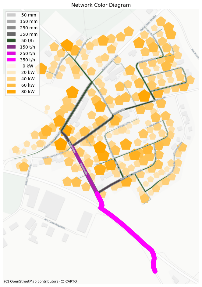
Network Color Diagram with matplotlib

fig, ax = plt.subplots(figsize=Rm.DINA3q)

nodes_patches_1 = ncd.pNcd_nodes(ax=ax,
                                 gdf=gdf_FWVB,
                                 attribute='W',  # kW
                                 colors=['oldlace', 'orange'],
                                 marker_style='p',
                                 legend_fmt='{:4.0f} kW',
                                 legend_values=[0, 20, 40, 60, 80],
                                 zorder=1)

pipes_patches_2 = ncd.pNcd_pipes(ax=ax,
                                 gdf=gdf_ROHR,
                                 attribute='DI',
                                 colors=['lightgray', 'dimgray'],
                                 legend_fmt='{:4.0f} mm',
                                 legend_values=[50, 150, 250, 350],
                                 zorder=2)

pipes_patches_3 = ncd.pNcd_pipes(ax=ax,
                                 gdf=gdf_ROHR,
                                 attribute='QMAVAbs',
                                 colors=['darkgreen', 'magenta'],
                                 legend_fmt='{:4.0f} t/h',
                                 legend_values=[50, 150, 250, 350],
                                 zorder=3)

all_patches = pipes_patches_2 + pipes_patches_3 + nodes_patches_1
ax.legend(handles=all_patches, loc='best')

cx.add_basemap(ax, crs=gdf_ROHR.crs.to_string(), source=cx.providers.CartoDB.PositronNoLabels)
cx.add_basemap(ax, crs=gdf_ROHR.crs.to_string(), source=cx.providers.CartoDB.PositronOnlyLabels)

plt.title('Network Color Diagram')

plt.savefig('Example1_Output_2.pdf', dpi=300, bbox_inches='tight')
plt.show()