Example 3: Longitudinal Sections
This example demonstrates how longitudinal sections data read by PT3S can be accessed and used to create plots with Matplotlib.
PT3S Release
[1]:
#pip install PT3S -U --no-deps
Necessary packages for this Example
When running this example for the first time on your machine, please execute the cell below. Afterward, you may need to restart the kernel (using the ‘fast-forward’ button).
[2]:
pip install -q bokeh
Note: you may need to restart the kernel to use updated packages.
Imports
[3]:
import os
import logging
import pandas as pd
import datetime
import numpy as np
import subprocess

import matplotlib
import matplotlib.pyplot as plt
import matplotlib.dates as mdates
import matplotlib.gridspec as gridspec
import matplotlib.ticker as ticker
import matplotlib.colors as mcolors
from matplotlib.pyplot import Polygon
from matplotlib.ticker import FuncFormatter
from matplotlib.dates import DateFormatter, MinuteLocator
import matplotlib.ticker as ticker

from bokeh.plotting import figure, show
from bokeh.io import output_notebook
from bokeh.models import CustomJS, ColumnDataSource, CheckboxGroup, LinearAxis, Range1d
from bokeh.layouts import column


try:
    from PT3S import dxAndMxHelperFcts
except:
    import dxAndMxHelperFcts

try:
    from PT3S import Rm
except:
    import Rm
[4]:
import importlib
from importlib import resources
[5]:
#importlib.reload(dxAndMxHelperFcts)
Logging
[6]:
logger = logging.getLogger()

if not logger.handlers:
    logFileName = r"Example3.log"
    loglevel = logging.DEBUG

    logging.basicConfig(
        filename=logFileName,
        filemode='w',
        level=loglevel,
        format="%(asctime)s ; %(name)-60s ; %(levelname)-7s ; %(message)s"
    )

    fileHandler = logging.FileHandler(logFileName)
    logger.addHandler(fileHandler)

    consoleHandler = logging.StreamHandler()
    consoleHandler.setFormatter(logging.Formatter("%(levelname)-7s ; %(message)s"))
    consoleHandler.setLevel(logging.INFO)
    logger.addHandler(consoleHandler)
Read Model and Results
[7]:
dbFilename="Example3"
dbFile = resources.files("PT3S").joinpath("Examples", f"{dbFilename}.db3")
[8]:
m=dxAndMxHelperFcts.readDxAndMx(dbFile=dbFile
                                ,preventPklDump=True
                                ,maxRecords=-1
                                ,mxsVecsResults2MxDfVecAggs=[7,13,19,-1]
                                #,SirCalcExePath=r"C:\3S\SIR 3S\SirCalc-90-14-02-12_Potsdam.fix1_x64\SirCalc.exe"
)
INFO    ; Dx.__init__: dbFile (abspath): c:\users\aUserName\3s\pt3s\PT3S\Examples\Example3.db3 exists readable ...
INFO    ; PT3S.dxAndMxHelperFcts.readDxAndMx:
+..\PT3S\Examples\Example3.db3 is newer than
+..\PT3S\Examples\WDExample3\B1\V0\BZ1\M-1-0-1.1.MX1:
+SIR 3S' dbFile is newer than SIR 3S' mx1File
+in this case the results are maybe dated or (worse) incompatible to the model
INFO    ; PT3S.dxAndMxHelperFcts.readDxAndMx: Model is being recalculated using C:\\3S\SIR 3S\SirCalc-90-15-02-26_Quebec.upd1\SirCalc.exe
INFO    ; Mx.setResultsToMxsFile: Mxs: ..\PT3S\Examples\WDExample3\B1\V0\BZ1\M-1-0-1.1.MXS reading ...
INFO    ; dxWithMx.__init__: Example3: processing dx and mx ...
Longitudinal Sections: V3_AGSN
[9]:
m.V3_AGSN.head()
[9]:
| Pos | pk | tk | LFDNR | NAME | XL | compNr | nextNODE | OBJTYPE | OBJID | ... | RHO_n | mlc_n | ('STAT', 'mlc', Timestamp('2023-02-12 23:00:00'), Timestamp('2023-02-12 23:00:00'))_n | ('TIME', 'mlc', Timestamp('2023-02-12 23:00:00'), Timestamp('2023-02-12 23:00:00'))_n | ('TMIN', 'mlc', Timestamp('2023-02-12 23:00:00'), Timestamp('2023-02-13 23:00:00'))_n | ('TMAX', 'mlc', Timestamp('2023-02-12 23:00:00'), Timestamp('2023-02-13 23:00:00'))_n | ('TIME', 'mlc', Timestamp('2023-02-13 06:00:00'), Timestamp('2023-02-13 06:00:00'))_n | ('TIME', 'mlc', Timestamp('2023-02-13 12:00:00'), Timestamp('2023-02-13 12:00:00'))_n | ('TIME', 'mlc', Timestamp('2023-02-13 18:00:00'), Timestamp('2023-02-13 18:00:00'))_n | ('TIME', 'mlc', Timestamp('2023-02-13 23:00:00'), Timestamp('2023-02-13 23:00:00'))_n | |
|---|---|---|---|---|---|---|---|---|---|---|---|---|---|---|---|---|---|---|---|---|---|
| 0 | -1 | 5755933101669454049 | 5755933101669454049 | 1.0 | Längsschnitt | 0 | 1 | V-E0 | ROHR | 5691533564979419761 | ... | 965.700012 | 592.989176 | 592.964637 | 592.964637 | 592.964666 | 603.808934 | 602.03647 | 599.224274 | 602.192273 | 593.485488 |
| 0 | 0 | 5755933101669454049 | 5755933101669454049 | 1.0 | Längsschnitt | 0 | 1 | V-K1683S | ROHR | 5691533564979419761 | ... | 965.701172 | 592.964637 | 592.964637 | 592.964637 | 592.964666 | 603.808934 | 602.03647 | 599.224274 | 602.192273 | 593.485488 |
| 1 | 1 | 5755933101669454049 | 5755933101669454049 | 1.0 | Längsschnitt | 0 | 1 | V-K1693S | ROHR | 5048873293262650113 | ... | 965.702148 | 592.944662 | 592.944662 | 592.944662 | 592.944715 | 603.734069 | 601.970656 | 599.172654 | 602.125668 | 593.462908 |
| 2 | 2 | 5755933101669454049 | 5755933101669454049 | 1.0 | Längsschnitt | 0 | 1 | V-K2163S | ROHR | 5715081934973525403 | ... | 965.702637 | 592.934654 | 592.934654 | 592.934654 | 592.934719 | 603.696568 | 601.937691 | 599.146793 | 602.0923 | 593.451594 |
| 3 | 3 | 5755933101669454049 | 5755933101669454049 | 1.0 | Längsschnitt | 0 | 1 | V-K2043S | ROHR | 5413647981880727734 | ... | 965.703735 | 592.911609 | 592.911609 | 592.911609 | 592.911702 | 603.610302 | 601.861849 | 599.087298 | 602.015548 | 593.425543 |
5 rows × 85 columns
Plot Section No. 1
Define Axes
[10]:
def fyPH(ax,offset=0):
    ax.spines["left"].set_position(("outward", offset))
    ax.set_ylabel('PH Druck in bar')
    #ax.set_ylim(1,6)
    #ax.set_yticks(sorted(np.append(np.linspace(1,6,11),[])))
    ax.yaxis.set_ticks_position('left')
    ax.yaxis.set_label_position('left')

def fymlc(ax,offset=60):
    ax.spines["left"].set_position(("outward", offset))
    ax.set_ylabel('mlc Druckhöhe in mlc')
    #ax.set_ylim(1,6)
    #ax.set_yticks(sorted(np.append(np.linspace(1,6,11),[])))
    ax.yaxis.set_ticks_position('left')
    ax.yaxis.set_label_position('left')

def fybarBzg(ax,offset=120):
    ax.spines["left"].set_position(("outward", offset))
    ax.set_ylabel('H Druck in barBzg')
    #ax.set_ylim(1,6)
    #ax.set_yticks(sorted(np.append(np.linspace(1,6,11),[])))
    ax.yaxis.set_ticks_position('left')
    ax.yaxis.set_label_position('left')

def fyM(ax,offset=180):
    Rm.pltLDSHelperY(ax)
    ax.spines["left"].set_position(("outward",offset))
    ax.set_ylabel('QM Massenstrom in t/h')
    #ax.set_ylim(500,550)
    #ax.set_yticks(sorted(np.append(np.linspace(500,550,11),[])))
    ax.yaxis.set_ticks_position('left')
    ax.yaxis.set_label_position('left')

def fyT(ax,offset=240):
    Rm.pltLDSHelperY(ax)
    ax.spines["left"].set_position(("outward",offset))
    ax.set_ylabel('T Tempertatur in °C')
    ax.set_ylim(55,95)
    #ax.set_yticks(sorted(np.append(np.linspace(0,95,11),[])))
    ax.yaxis.set_ticks_position('left')
    ax.yaxis.set_label_position('left')
Plotfunction
[11]:
def plot(dfAGSN=pd.DataFrame()
        ,dfAGSNRL=pd.DataFrame()
        ,PHCol='PH_n'
        ,mlcCol='mlc_n'
        ,zKoorCol='ZKOR_n'
        ,barBzgCol='H_n'
        ,QMCol='QM'
        ,TCol='T_n'
        ,xCol='LSum'

):

    fig, ax0 = plt.subplots(figsize=Rm.DINA3q)

    ax0.set_yticks(np.linspace(0, 10, 21))
    ax0.yaxis.set_ticklabels([])
    ax0.grid()

    #PH
    ax1 = ax0.twinx()
    fyPH(ax1)
    PH_SL=ax1.plot(dfAGSN[xCol], dfAGSN[PHCol], color='red', label='PH SL',ls='dotted')
    PH_RL=ax1.plot(dfAGSNRL[xCol], dfAGSNRL[PHCol], color='blue', label='PH RL',ls='dotted')

    #mlc
    ax11 = ax0.twinx()
    fymlc(ax11)
    mlc_SL=ax11.plot(dfAGSN[xCol], dfAGSN[mlcCol], color='red', label='mlc SL')
    mlc_RL=ax11.plot(dfAGSNRL[xCol], dfAGSNRL[mlcCol], color='blue', label='mlc RL')

    z=ax11.plot(dfAGSN[xCol], dfAGSN[zKoorCol], color='black', label='z',ls='dashed',alpha=.5)

    #barBZG
    ax12 = ax0.twinx()
    fybarBzg(ax12)
    barB_SL=ax12.plot(dfAGSN[xCol], dfAGSN[barBzgCol], color='red', label='H SL',ls='dashdot')
    barB_RL=ax12.plot(dfAGSNRL[xCol], dfAGSNRL[barBzgCol], color='blue', label='H RL',ls='dashdot')

    #M
    ax2 = ax0.twinx()
    fyM(ax2)
    QM_SL=ax2.step(dfAGSN[xCol], dfAGSN[QMCol]*dfAGSN['direction'], color='orange', label='M SL')
    QM_RL=ax2.step(dfAGSNRL[xCol], dfAGSNRL[QMCol]*dfAGSNRL['direction'], color='cyan', label='M RL',ls='--')

    #T
    ax3 = ax0.twinx()
    fyT(ax3)
    T_SL=ax3.plot(dfAGSN[xCol], dfAGSN[TCol], color='pink', label='T SL')
    T_RL=ax3.plot(dfAGSNRL[xCol], dfAGSNRL[TCol], color='lavender', label='T RL')

    ax0.set_title('Longitudinal Section for '+dbFilename)

    # added these three lines
    lns =  PH_SL+ PH_RL + mlc_SL+ mlc_RL + barB_SL+ barB_RL+ QM_SL+ QM_RL + T_SL+ T_RL + z
    labs = [l.get_label() for l in lns]
    ax0.legend(lns, labs)#, loc=0)

    plt.show()
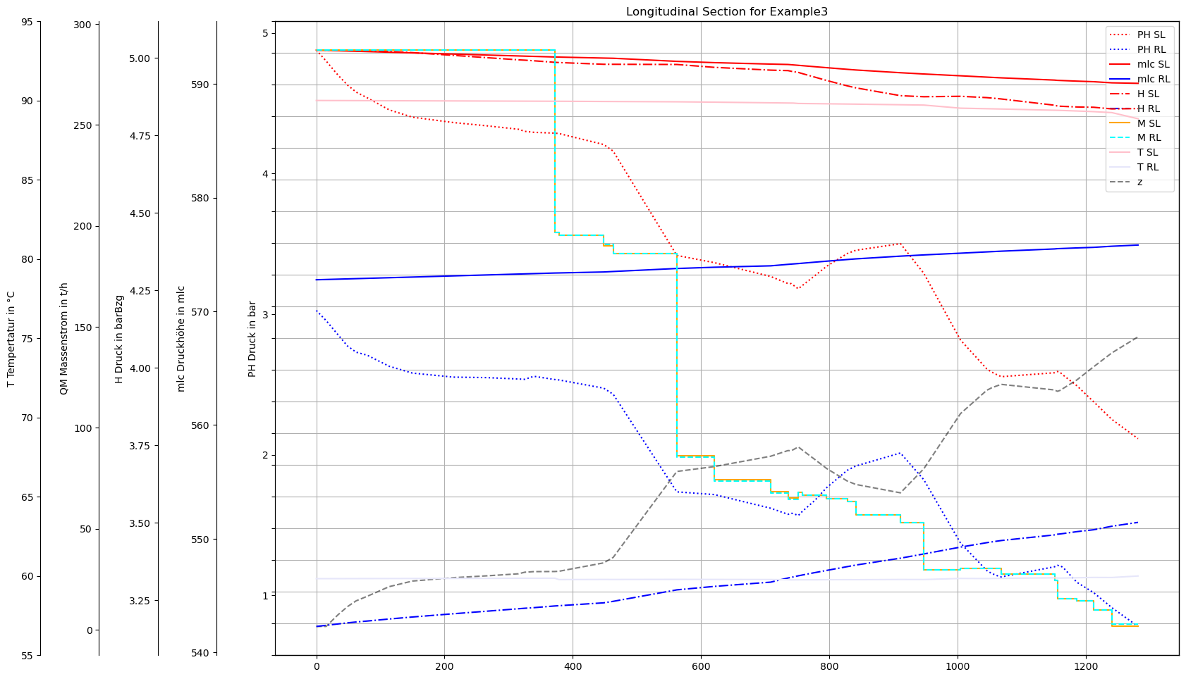
Plot without vector data
[12]:
dfAGSN=m.V3_AGSN[
    (m.V3_AGSN['LFDNR']==1)
    &
    (m.V3_AGSN['XL']==1)
]
[13]:
dfAGSNRL=m.V3_AGSN[
    (m.V3_AGSN['LFDNR']==1)
    &
    (m.V3_AGSN['XL']==2)
]
[14]:
plot(dfAGSN,dfAGSNRL)
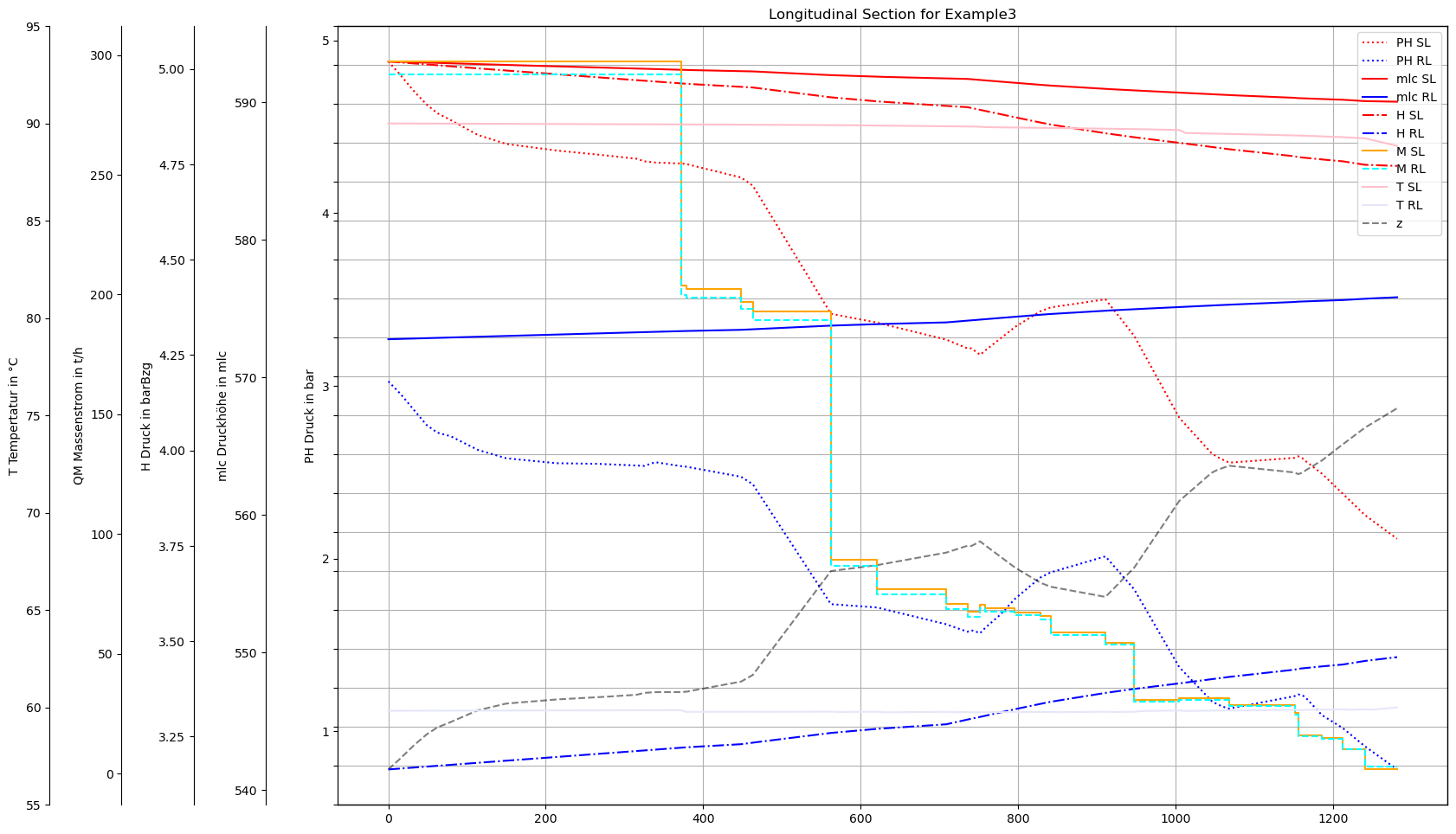
Plot with vector data (with pipe interior points)
[15]:
dfAGSNVec=m.V3_AGSNVEC[
    (m.V3_AGSNVEC['LFDNR']==1)
    &
    (m.V3_AGSNVEC['XL']==1)
]
[16]:
dfAGSNVecRL=m.V3_AGSNVEC[
 (m.V3_AGSNVEC['LFDNR']==1)
    &
    (m.V3_AGSNVEC['XL']==2)
]
[17]:
t0rVec=pd.Timestamp(m.mx.df.index[0].strftime('%Y-%m-%d %X'))#.%f'))
[18]:
manPVEC=('STAT',
                      'manPVEC',
                      t0rVec,
                      t0rVec)
[19]:
manPVEC
[19]:
('STAT',
 'manPVEC',
 Timestamp('2023-02-12 23:00:00'),
 Timestamp('2023-02-12 23:00:00'))
[20]:
# for convenient colnames in celloutput
dfAGSNVec['manPVEC']=dfAGSNVec[manPVEC]
dfAGSNVecRL['manPVEC']=dfAGSNVecRL[manPVEC]
[21]:
mlcPVEC=('STAT',
                      'mlcPVEC',
                      t0rVec,
                      t0rVec)
[22]:
# for convenient colnames in celloutput
dfAGSNVec['mlcPVEC']=dfAGSNVec[mlcPVEC]
dfAGSNVecRL['mlcPVEC']=dfAGSNVecRL[mlcPVEC]
[23]:
QMVEC=('STAT',
                      'QMVEC',
                      t0rVec,
                      t0rVec)
[24]:
QMVEC=('STAT',
                      'QMVEC',
                      t0rVec,
                      t0rVec)
[25]:
# for convenient colnames in celloutput
dfAGSNVec['QMVEC']=dfAGSNVec[QMVEC]
dfAGSNVecRL['QMVEC']=dfAGSNVecRL[QMVEC]
[26]:
TVEC=('STAT',
'ROHR~*~*~*~TVEC',
t0rVec,
t0rVec)
[27]:
# for convenient colnames in celloutput
dfAGSNVec['TVEC']=dfAGSNVec[TVEC]
dfAGSNVecRL['TVEC']=dfAGSNVecRL[TVEC]
[28]:
plot(dfAGSNVec,dfAGSNVecRL
        ,PHCol=manPVEC
        ,mlcCol=mlcPVEC
        ,zKoorCol='ZVEC'
        ,barBzgCol='H_n'
        ,QMCol=QMVEC
        ,TCol=TVEC
        ,xCol='LSum'

    )
Plot different timesteps with Bokeh
[29]:
def bokeh_plot(df, x_col, y_cols, y2_cols, y3_cols):
    output_notebook()

    p = figure(width=1366, height=768, title="Longitudinal Section for "+dbFilename+" at different timestamps", x_axis_label=x_col, y_axis_label="PH Druck in bar", tools="pan,wheel_zoom,box_zoom,reset", y_range=Range1d(start=0, end=6))

    # Define line styles and colors
    line_styles = ['solid', 'dashed', 'dotted']
    colors = ['blue', 'red', 'green']
    lines = []

    # lines for y
    for i, y_col in enumerate(y_cols):
        line = p.line(df[x_col], df[y_col], legend_label=f"{y_col} (06:00)" if i == 0 else f"{y_col} (12:00)" if i == 1 else f"{y_col} (18:00)", line_width=2, line_dash=line_styles[i % len(line_styles)], color=colors[0])
        lines.append(line)

    #second y-axis
    p.extra_y_ranges = {"y2": Range1d(start=0, end=600)}
    p.add_layout(LinearAxis(y_range_name="y2", axis_label="QM Massenstrom in t/h"), 'left')

    # lines for y2
    for i, y2_col in enumerate(y2_cols):
        line = p.line(df[x_col], df[y2_col], legend_label=f"{y2_col} (06:00)" if i == 0 else f"{y2_col} (12:00)" if i == 1 else f"{y2_col} (18:00)", line_width=2, line_dash=line_styles[i % len(line_styles)], color=colors[1], y_range_name="y2")
        lines.append(line)

    #third y-axis
    p.extra_y_ranges["y3"] = Range1d(start=590, end=610)
    p.add_layout(LinearAxis(y_range_name="y3", axis_label="mlc in m"), 'left')

    # lines for y3
    for i, y3_col in enumerate(y3_cols):
        line = p.line(df[x_col], df[y3_col], legend_label=f"{y3_col} (06:00)" if i == 0 else f"{y3_col} (12:00)" if i == 1 else f"{y3_col} (18:00)", line_width=2, line_dash=line_styles[i % len(line_styles)], color=colors[2], y_range_name="y3")
        lines.append(line)

    # Create a CheckboxGroup
    labels = [f"{y_col}" for i, y_col in enumerate(y_cols + y2_cols + y3_cols)]
    checkbox = CheckboxGroup(labels=labels, active=list(range(len(labels))))

    # CustomJS to toggle visibility
    checkbox.js_on_change('active', CustomJS(args=dict(lines=lines), code="""
        for (let i = 0; i < lines.length; i++) {
            lines[i].visible = this.active.includes(i);
        }
    """))

    show(column(p, checkbox))
[30]:
bokeh_plot(dfAGSNVec, 'LSum',['PH_n_1', 'PH_n_2', 'PH_n_3'], ['QM_1', 'QM_2', 'QM_3'], ['mlc_n_1', 'mlc_n_2', 'mlc_n_3'])
[31]:
m.V3_AGSNVEC
[31]:
| Pos | pk | tk | LFDNR | NAME | XL | compNr | nextNODE | OBJTYPE | OBJID | ... | mlc_n_1 | QM_1 | T_n_2 | PH_n_2 | mlc_n_2 | QM_2 | T_n_3 | PH_n_3 | mlc_n_3 | QM_3 | |
|---|---|---|---|---|---|---|---|---|---|---|---|---|---|---|---|---|---|---|---|---|---|
| 0 | 0 | 5755933101669454049 | 5755933101669454049 | 1.0 | Längsschnitt | 0 | 1 | V-E0 | ROHR | 5691533564979419761 | ... | 602.117263 | 529.095026 | 90.000000 | 5.475470 | 599.287638 | 467.313519 | 90.000000 | 5.758390 | 602.274067 | 532.336816 |
| 1 | 0 | 5755933101669454049 | 5755933101669454049 | 1.0 | Längsschnitt | 0 | 1 | V-K1683S | ROHR | 5691533564979419761 | ... | 602.076878 | 529.095026 | 89.999390 | 5.434580 | 599.256014 | 467.313519 | 89.999481 | 5.716620 | 602.233160 | 532.336816 |
| 2 | 0 | 5755933101669454049 | 5755933101669454049 | 1.0 | Längsschnitt | 0 | 1 | V-K1683S | ROHR | 5691533564979419761 | ... | 602.036490 | 529.095026 | 89.998779 | 5.393685 | 599.224279 | 467.313519 | 89.998932 | 5.674860 | 602.192293 | 532.336816 |
| 3 | 1 | 5755933101669454049 | 5755933101669454049 | 1.0 | Längsschnitt | 0 | 1 | V-K1693S | ROHR | 5048873293262650113 | ... | 602.003598 | 529.095026 | 89.998291 | 5.358085 | 599.198512 | 467.313519 | 89.998505 | 5.638545 | 602.158983 | 532.336816 |
| 4 | 1 | 5755933101669454049 | 5755933101669454049 | 1.0 | Längsschnitt | 0 | 1 | V-K1693S | ROHR | 5048873293262650113 | ... | 601.970651 | 529.095026 | 89.997803 | 5.322480 | 599.172633 | 467.313519 | 89.998077 | 5.602235 | 602.125663 | 532.336816 |
| ... | ... | ... | ... | ... | ... | ... | ... | ... | ... | ... | ... | ... | ... | ... | ... | ... | ... | ... | ... | ... | ... |
| 1768 | 43 | 4868980900521118307 | 4868980900521118307 | 3.0 | Längsschnitt in bar,B | 2 | 1 | R-K2623S | ROHR | 4814824415166736381 | ... | 582.416769 | -5.052247 | 59.929230 | 1.329900 | 580.358716 | -4.463768 | 59.937866 | 1.539505 | 582.530757 | -5.082847 |
| 1769 | 43 | 4868980900521118307 | 4868980900521118307 | 3.0 | Längsschnitt in bar,B | 2 | 1 | R-K2623S | ROHR | 4814824415166736381 | ... | 582.481984 | -5.052247 | 59.946930 | 1.306120 | 580.410458 | -4.463768 | 59.953400 | 1.517095 | 582.596697 | -5.082847 |
| 1770 | 43 | 4868980900521118307 | 4868980900521118307 | 3.0 | Längsschnitt in bar,B | 2 | 1 | R-K2623S | ROHR | 4814824415166736381 | ... | 582.547134 | -5.052247 | 59.964630 | 1.282340 | 580.462136 | -4.463768 | 59.968933 | 1.494685 | 582.662573 | -5.082847 |
| 1771 | 43 | 4868980900521118307 | 4868980900521118307 | 3.0 | Längsschnitt in bar,B | 2 | 1 | R-K2623S | ROHR | 4814824415166736381 | ... | 582.612344 | -5.052247 | 59.982300 | 1.258565 | 580.513921 | -4.463768 | 59.984467 | 1.472280 | 582.728560 | -5.082847 |
| 1772 | 43 | 4868980900521118307 | 4868980900521118307 | 3.0 | Längsschnitt in bar,B | 2 | 1 | R-K2623S | ROHR | 4814824415166736381 | ... | 582.677538 | -5.052247 | 60.000000 | 1.234785 | 580.565589 | -4.463768 | 60.000000 | 1.449870 | 582.794427 | -5.082847 |
1773 rows × 596 columns